From scratch on TPU v5e: training mammography classifiers in JAX/Flax
This is a write-up of the TPU portion of my undergraduate thesis (CM3070, Computer Science Final Project, University of London Goldsmiths). The thesis built two parallel pipelines for the same task: patch-level classification on the Curated Breast Imaging Subset of DDSM. Across both pipelines I trained 15 deep-learning experiments on a Google Cloud v5litepod-8 TPU v5e accelerator using JAX/Flax. The TPU pipeline is on GitHub: CM3070-Models-Training-with-TPUs.
The post focuses on the JAX/Flax/TPU pipeline. A separate PyTorch pipeline handled pretrained models and explainability, and that one is a story for another day.
The setup
The dataset is curated_breast_imaging_ddsm/patches:3.0.0, distributed via TensorFlow Datasets. Each example is a 224 x 224 single-channel mammographic patch with one of five labels: BACKGROUND, BENIGN_CALCIFICATION, BENIGN_MASS, MALIGNANT_CALCIFICATION, MALIGNANT_MASS. The splits are fixed at 49,780 train / 5,580 validation / 9,770 test samples.
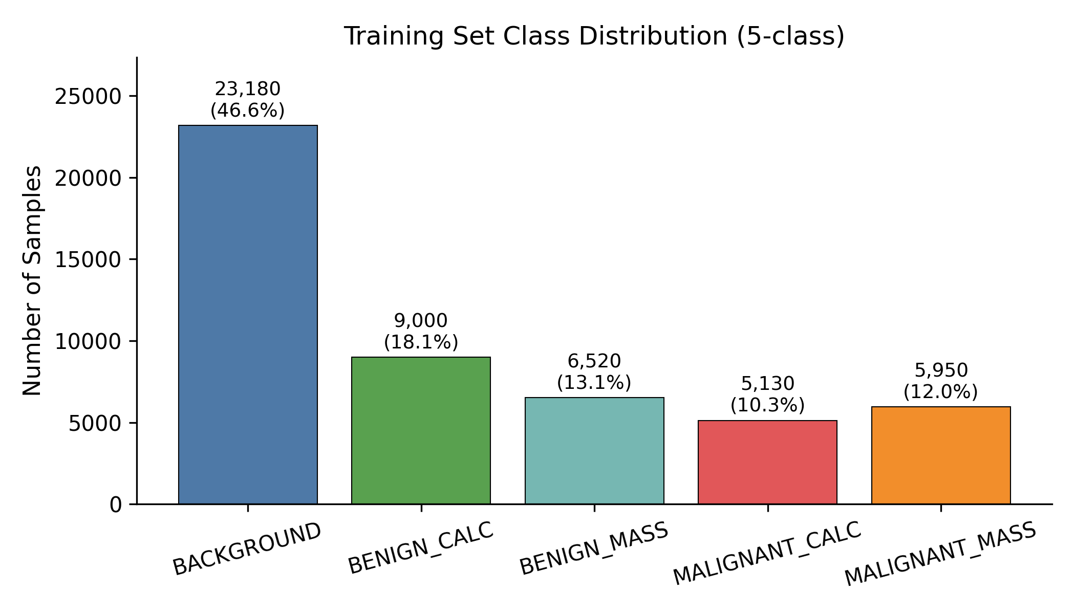
The class imbalance shapes everything that follows: BACKGROUND alone is 46.6% of the training set, while the two malignant classes together are 22.3%. Balanced accuracy and macro-F1 are the metrics that matter; raw accuracy can always be hacked by predicting BACKGROUND more often.
Why TPU, and why JAX
This was a deliberate “learning by doing” choice. The PyTorch ecosystem is more mature for medical imaging, has timm for pretrained backbones, has pytorch-grad-cam for explainability, and has a clean ONNX export path. JAX has none of those out of the box. But JAX gives you pmap, jit, fully functional state, and a TPU programming model that is genuinely fun to write. On top of that, TPU v5e is significantly cheaper per FLOP than equivalent GPU options if you can stomach the rougher tooling.
So the TPU pipeline runs from random initialisation. No pretrained weights. The whole point was to see how far a from-scratch model can go on a constrained dataset, and what “training a model on a TPU pod” actually feels like end-to-end: provisioning, data on GCS, multi-host data parallelism, checkpointing, the lot.
The pipeline
The training loop is built around jax.pmap on a v5litepod-8 slice: 8 TPU v5e chips, one TensorCore per chip, 16 GB HBM per chip for 128 GB total. JAX sees 8 devices, and pmap shards the global batch across all of them. Mixed precision is bfloat16 throughout, AdamW + warmup-cosine, gradient norm clipped at 1.0, Orbax for checkpointing. A typical run config looks like this (the final_best ResNet34 recipe):
# resnet34_gray model
stage_sizes: [3, 4, 6, 3]
widths: [64, 128, 256, 512]
in_channels: 1
dropout_rate: 0.1
stochastic_depth_rate: 0.05

# training
seed: 21
epochs: 35
batch_size: 256          # global, sharded 8-way across cores
learning_rate: 0.0007
warmup_epochs: 3
weight_decay: 0.0002
optimizer: adamw
loss_name: focal
class_weights: [0.5, 1.0, 1.0, 1.3, 1.3]
label_smoothing: 0.03
dropout_rate_override: 0.15
ema_decay: 0.999
use_bfloat16: true
grad_clip_norm: 1.0
selection_metric: macro_f1
A guided tour of the JAX code
Before showing the train step, it’s worth walking through the building blocks the loop assembles. Each one is short (the TPU project’s training package is under 850 lines of Python), and reading them top-down gives a fair sense of how JAX, Flax, and Optax fit together.
1. The learning-rate schedule is one Optax call. It’s a pure function step -> lr, so the optimizer can ask for the LR at any step without keeping side state:
# src/breast_patch_cls/training/lr_schedules.py
def create_learning_rate_schedule(config: TrainConfig, steps_per_epoch: int):
    warmup_steps = config.warmup_epochs * steps_per_epoch
    total_steps  = config.epochs * steps_per_epoch
    return optax.warmup_cosine_decay_schedule(
        init_value=0.0,
        peak_value=config.learning_rate,
        warmup_steps=warmup_steps,
        decay_steps=max(total_steps - warmup_steps, 1),
        end_value=0.0,
    )
2. The optimizer is just a chain of pure transformations. Optax expresses every optimizer as (grads, state) -> (updates, new_state), and optax.chain composes any number of those transformations into a single one. Here gradient clipping happens before AdamW, which is what you almost always want on TPU because clipping after the parameter update is too late to help with the occasional bf16 spike:
# src/breast_patch_cls/training/optimizer.py
def create_optimizer(config: TrainConfig, learning_rate_schedule):
    transforms = []
    if config.grad_clip_norm is not None:
        transforms.append(optax.clip_by_global_norm(config.grad_clip_norm))
    if config.optimizer == "adamw":
        transforms.append(
            optax.adamw(
                learning_rate=learning_rate_schedule,
                weight_decay=config.weight_decay,
            )
        )
    return optax.chain(*transforms)
3. Focal loss in five lines. This is the kind of code that tells you why the JAX style is fun. There is no jit, no pmap, no shape juggling, no device placement: just jnp ops on logits and a one-hot target. The compilation and parallelism happen later, when the training step closes over this function:
# src/breast_patch_cls/training/losses.py
def _softmax_focal_loss(logits, one_hot, gamma=2.0):
    log_probs = jax.nn.log_softmax(logits)
    probs     = jnp.exp(log_probs)
    pt        = jnp.sum(probs * one_hot, axis=-1)
    ce        = -jnp.sum(log_probs * one_hot, axis=-1)
    return ((1.0 - pt) ** gamma) * ce
The full classification_loss wraps this with optional label smoothing (optax.smooth_labels) and per-class weights. Class weighting is a single broadcast: losses = losses * class_weights[labels]. No nn.CrossEntropyLoss(weight=...) ceremony.
4. The Flax model is a linen.Module. Flax modules are dataclasses with a __call__ defined under @nn.compact. The train flag flips BatchNorm and Dropout into eval mode at evaluation time. Conv / BN / ReLU is recognisable to anyone coming from PyTorch, but the call site is different: you don’t see .cuda() or .to(device) anywhere because devices live outside the model:
# src/breast_patch_cls/models/resnet.py
class ResNetBlock(nn.Module):
    features: int
    stride: int = 1
    drop_path_rate: float = 0.0
    dtype: jnp.dtype = jnp.float32

    @nn.compact
    def __call__(self, x, *, train: bool):
        residual = x
        x = nn.Conv(self.features, (3, 3), self.stride,
                    padding="SAME", use_bias=False, dtype=self.dtype)(x)
        x = nn.BatchNorm(use_running_average=not train,
                         momentum=0.9, epsilon=1e-5)(x)
        x = nn.relu(x)
        x = nn.Conv(self.features, (3, 3), 1,
                    padding="SAME", use_bias=False, dtype=self.dtype)(x)
        x = nn.BatchNorm(use_running_average=not train,
                         momentum=0.9, epsilon=1e-5,
                         scale_init=nn.initializers.zeros_init())(x)
        if residual.shape != x.shape:
            residual = nn.Conv(self.features, (1, 1), self.stride,
                               use_bias=False, dtype=self.dtype)(residual)
            residual = nn.BatchNorm(use_running_average=not train,
                                    momentum=0.9, epsilon=1e-5)(residual)
        x = DropPath(self.drop_path_rate)(x, deterministic=not train)
        return nn.relu(x + residual)
The zero-init on the second BatchNorm scale is the classic “identity at init” trick: each block starts out as the identity function, which makes deep ResNets train more stably from random weights. That stability matters a lot when you’re going from-scratch instead of fine-tuning.
5. The whole training state is one pytree. This is the line where Flax and JAX’s design earns the most credit. Optimizer state, EMA params, BatchNorm running stats, and the dropout RNG all sit in one TrainState object:
# src/breast_patch_cls/training/train_state.py
class TrainState(train_state.TrainState):
    batch_stats: PyTree | None = None
    ema_params:  PyTree | None = None
    rng:         PyTree | None = struct.field(pytree_node=True, default=None)
flax.jax_utils.replicate(state) puts a copy on every device. flax.jax_utils.unreplicate(state) brings one back to the host. Save the pytree and you have saved the whole run; load it and you can resume. There is no separate “optimizer.pt + model.pt + scheduler.pt + scaler.pt” dance, and no question about which device each piece lives on.
With those five pieces in hand, the training step is just gluing them together. Gradients, batch-stats, and EMA updates are all pmean‘d across the batch axis:
def train_step(state, batch):
    dropout_rng, next_rng = jax.random.split(state.rng)
    dropout_rng = jax.random.fold_in(dropout_rng, jax.lax.axis_index("batch"))

    def loss_fn(params):
        variables = _state_variables(state) | {"params": params}
        logits, updates = model.apply(
            variables, batch["image"], train=True,
            rngs={"dropout": dropout_rng},
            mutable=["batch_stats"],
        )
        loss = classification_loss(logits, batch["label"], cfg, num_classes)
        return loss, (logits, updates["batch_stats"])

    (loss, (logits, new_bs)), grads = jax.value_and_grad(loss_fn, has_aux=True)(state.params)
    grads = jax.lax.pmean(grads, axis_name="batch")
    loss  = jax.lax.pmean(loss,  axis_name="batch")
    new_state = state.apply_gradients(grads=grads).replace(
        batch_stats=jax.lax.pmean(new_bs, axis_name="batch"),
        rng=next_rng,
    )
    if cfg.ema_decay is not None:
        ema = jax.tree_util.tree_map(
            lambda o, n: cfg.ema_decay * o + (1.0 - cfg.ema_decay) * n,
            state.ema_params, new_state.params,
        )
        new_state = new_state.replace(ema_params=ema)
    return new_state, {"loss": loss}
Once you’re comfortable with the functional state pattern, this style of training loop is honestly delightful. Every transformation is a pure function, and the pmap boundary makes data parallelism explicit instead of magical.
Living with JAX/Flax on TPU
It’s worth digging into what the stack actually feels like in practice, because most “JAX vs PyTorch” takes online are abstract and not very useful when you’re 30 minutes into a TPU lease and your loss is nan.
Functional state, on purpose
In PyTorch, a model is a stateful object. You call .to(device), .train(), .zero_grad(), and parameters mutate in place. In Flax (the older linen API I used here), a model is a description: model.init(rng, x) runs the forward once and returns a frozen pytree of parameters and buffers. From then on, every step is params -> grads -> new_params, all explicit, all immutable.
That sounds bureaucratic until you realise what it buys you. The optimizer state, EMA weights, BatchNorm running stats, and dropout RNG are all just additional pytrees inside one TrainState. Replicating the whole thing across 8 chips is one call:
replicated_state = flax.jax_utils.replicate(state)
Saving a checkpoint is “serialise this pytree.” Restoring is “load this pytree.” There is no gnarly question about which device the optimizer state lives on, or whether .cuda() was called in the right order. That mental simplicity is the single biggest reason I kept reaching for JAX even when the surrounding ecosystem hurt.
pmap is the whole game on a single host
jax.pmap is conceptually vmap-with-side-effects: it adds a leading device axis and runs the function on each device in parallel. Anything you mark with axis_name="batch" gets a cross-device collective at that point. In our train step, three things cross the device boundary:
jax.lax.pmean(grads, axis_name="batch"): average gradients across all 8 chips so every replica steps to the same new params.jax.lax.pmean(loss, axis_name="batch"): purely for logging; doesn’t affect training.jax.lax.pmean(new_batch_stats, axis_name="batch"): sync BatchNorm running mean/var so they don’t drift per replica.
EMA is updated after the pmean, so it stays in lockstep automatically. The dropout_rng is fold_in‘d with jax.lax.axis_index("batch") so each replica gets a different dropout mask without us having to thread separate RNGs by hand.
Once that pattern clicks, single-host data parallelism stops being a thing you think about. You write your step function as if the batch were just (B/8, ...) and let pmap deal with the rest.
bfloat16 is free, mostly
TPU v5e’s matrix unit (MXU) is built for bfloat16. We compute in bf16, accumulate in fp32, and keep the optimizer state in fp32. In Flax this is a model-side choice: pass param_dtype=jnp.float32, dtype=jnp.bfloat16 to the conv/dense modules and Flax casts on the fly. Gradients come back in fp32 because the optimizer state is fp32, so AdamW updates stay numerically clean.
What surprised me on this dataset: I never hit a single nan/inf from bf16 alone. The two times the loss exploded it was because of a bad LR (focal loss + 7e-4 + no warmup) or a bad augmentation magnitude, not from the precision. Gradient clipping at norm 1.0 is the cheap insurance policy.
XLA compilation is real wall-clock
The first time you run a pmap‘d step, JAX traces the function, compiles it through XLA, and ships the compiled HLO to the chips. On v5e for a ResNet34 forward+backward at batch 256, this took roughly 60–90 seconds before the first step actually executed. Subsequent steps are blazing.
Two practical consequences:
- Don’t change shapes. Every shape change retriggers compilation. The data pipeline has to produce a fixed
(local_devices, B/local_devices, H, W, C)shape forever, which is whydrop_remainder=Trueis set on every dataset and why the test set is effectively 9,728 samples instead of 9,770. - Smoke-test on CPU first. I ran
configs/experiments/smoke_small_cnn.yamlon a laptop before every TPU session. Catching a Flax module bug after a 90-second compile on a chip you’re paying for by the minute is its own special kind of pain.
Data: TFDS over GCS, no tf.distribute involved
The dataset lives in a public Google Cloud Storage bucket (gs://cm3070-davidc-cbis-ddsm/tfds) as a sharded TFDS build of curated_breast_imaging_ddsm/patches:3.0.0. From the TPU VM’s point of view, “where is the data” is just a config field:
# configs/data/conservative_aug.yaml
dataset_name: curated_breast_imaging_ddsm/patches:3.0.0
data_dir: gs://cm3070-davidc-cbis-ddsm/tfds
train_split: train
validation_split: validation
test_split: test
image_size: [224, 224, 1]
shuffle_buffer_size: 8192
prefetch_batches: 4
drop_remainder: true
TFDS gives you two entry points and we use both. tfds.builder(...) is the metadata side (number of examples per split, feature schemas), useful for sizing steps_per_epoch without scanning the dataset:
# src/breast_patch_cls/data/tfds_builder.py
def load_builder(config: DataConfig) -> tfds.core.DatasetBuilder:
    return tfds.builder(config.dataset_name, data_dir=config.data_dir)

# elsewhere:
builder = load_builder(config.data)
train_examples = builder.info.splits[config.data.train_split].num_examples
steps_per_epoch = train_examples // config.train.batch_size
tfds.load(...) is the data side. It returns a tf.data.Dataset of decoded examples, which we then plug into a small tf.data pipeline doing shuffle / preprocess / augment / batch / prefetch:
# src/breast_patch_cls/data/input_pipeline.py
def make_dataset(config, *, split, batch_size, training, limit_steps=None):
    ds = tfds.load(config.dataset_name, split=split, data_dir=config.data_dir)
    options = tf.data.Options()
    options.experimental_deterministic = not training
    ds = ds.with_options(options)

    if config.cache:
        ds = ds.cache()
    if training:
        ds = ds.shuffle(config.shuffle_buffer_size, reshuffle_each_iteration=True)

    ds = ds.map(lambda ex: preprocess_example(ex, config),
                num_parallel_calls=tf.data.AUTOTUNE)
    if training:
        ds = ds.map(
            lambda ex: {"image": augment_image(ex["image"], config.augmentation),
                        "label": ex["label"], "id": ex["id"]},
            num_parallel_calls=tf.data.AUTOTUNE,
        )
        ds = ds.repeat()

    ds = ds.batch(batch_size, drop_remainder=True)
    return ds.prefetch(config.prefetch_batches)
A few things worth highlighting for anyone setting up a TPU pipeline for the first time:
drop_remainder=Trueis non-negotiable. TPU/XLA needs static shapes. A trailing partial batch would either retrigger compilation or crash. The cost is that the test set is effectively 9,728 samples instead of 9,770 (the 42-sample residual gets dropped), small enough that test metrics shift by < 0.1 pp.AUTOTUNEon host CPU is enough. Augmentation runs intf.dataon the host, not on the TPU. The chips never see uint8 inputs; by the time a batch reaches them it’s already float, normalised, augmented, and pre-sharded.reshuffle_each_iteration=Trueis the difference between “every epoch sees the same shuffle” and a different one. Easy to miss; matters more than you’d think for small datasets.
Preprocessing and augmentation are plain TensorFlow ops. Normalisation is parameterised by config (mean_std or minus_one_to_one):
# src/breast_patch_cls/data/preprocessing.py
def normalize_image(image, config):
    image = tf.cast(image, tf.float32) / 255.0
    if config.normalization.mode == "mean_std":
        return (image - config.normalization.mean) / config.normalization.std
    if config.normalization.mode == "minus_one_to_one":
        return image * 2.0 - 1.0
    raise ValueError(f"Unsupported normalization mode: {config.normalization.mode}")
The augmentation lives in data/augmentations.py. Translation is a tf.roll with a uniform random shift; rotation is a small affine transform via tf.raw_ops.ImageProjectiveTransformV3; brightness and contrast are stock tf.image ops. Horizontal flip is gated by config (default off) because mammographic patches carry left/right diagnostic information, and the conservative recipe deliberately keeps the magnitudes tiny (6-pixel translation, 10° rotation, brightness δ = 0.05). The augmentation ablation later in this post shows why being conservative was the right call.
The bridge from tf.data to JAX is one helper that calls tfds.as_numpy and yields plain NumPy dicts:
# src/breast_patch_cls/data/input_pipeline.py
def dataset_iterator(dataset: tf.data.Dataset):
    for batch in tfds.as_numpy(dataset):
        yield {"image": batch["image"], "label": batch["label"], "id": batch["id"]}
That iterator is then wrapped by prepare_per_device_iterator, which adds the (local_devices, B/local_devices, …) reshape and prefetches host batches onto the TPU using flax.jax_utils.prefetch_to_device. The TFDS / tf.data half stays on the host CPU; everything past the reshape is JAX’s.
There’s no tf.distribute.TPUStrategy anywhere. The TPU runtime is JAX’s; TFDS and tf.data are purely host-side. This split (TF for I/O, JAX for compute) turns out to be much less painful than the all-TF setups I’d seen described in older blog posts, and it means the same data pipeline works unchanged when I run a smoke test on a laptop with jax.local_device_count() == 1.
Orbax checkpointing in two lines
Saving the full TrainState to GCS is one call to orbax.CheckpointManager. Restoring is another. The painful step is making sure the pytree structure you’re restoring into matches what was saved (Flax module changes can break this). I found that pinning the model class and config alongside the checkpoint paid for itself the first time I came back to a run a week later and couldn’t remember whether the EMA weights were on or off.
Where the friction lives
Everything I wrote above is the good part. The honest pain points were:
- Pretrained weights.
timmdoesn’t exist for JAX. There are scenic and big_vision, but the parameter-mapping work to import an ImageNet ResNet50’s pretrained weights into a custom FlaxlinenResNet is meaningful. I decided to skip it and go from-scratch, which is in retrospect part of why the TPU numbers trail the GPU numbers by 10 pp. - ONNX export. No first-class path. The pragmatic approach is
jax2tfto atf.SavedModel, thentf2onnx. Two-step, fragile, and I never bothered. - Explainability.
pytorch-grad-camhas no JAX equivalent that’s as turnkey. You can write GradCAM in JAX (gradients of class score w.r.t. activations is, after all, exactly what JAX is good at), but for the explainability section of the thesis it was clearly the right call to switch to PyTorch. - Error messages. XLA traceback errors on a compile failure are notoriously bad. “Invalid argument: Expected shape …” with 80 lines of MLIR is not a fun debugging experience. The fix in 90% of cases is “trace through your shapes by hand on CPU first.”
The summary I’d give to anyone considering JAX on TPU for a research-scale project: if your problem is a custom training loop, an architecture you control end-to-end, and lots of compute to burn, JAX is wonderful. If your problem is fine-tune-this-pretrained-model-and-explain-its-decisions, pick PyTorch and be home for dinner.
What I trained
Five architectures, all from random initialisation:
- SmallCNN: a 4-block convnet, used only as a smoke test for the pipeline.
- ResNet18 / ResNet34 / ResNet50: adapted for grayscale (5×5 stride-2 stem), GroupNorm/BatchNorm, stochastic depth at 0.05 drop-path.
- ViT-Tiny / ViT-Small: 16×16 patch embedding, learnable positional embeddings, [CLS] token.
Across the five architectures plus a tuning campaign on ResNet34 plus a hyperparameter ablation, I shipped 15 TPU runs.
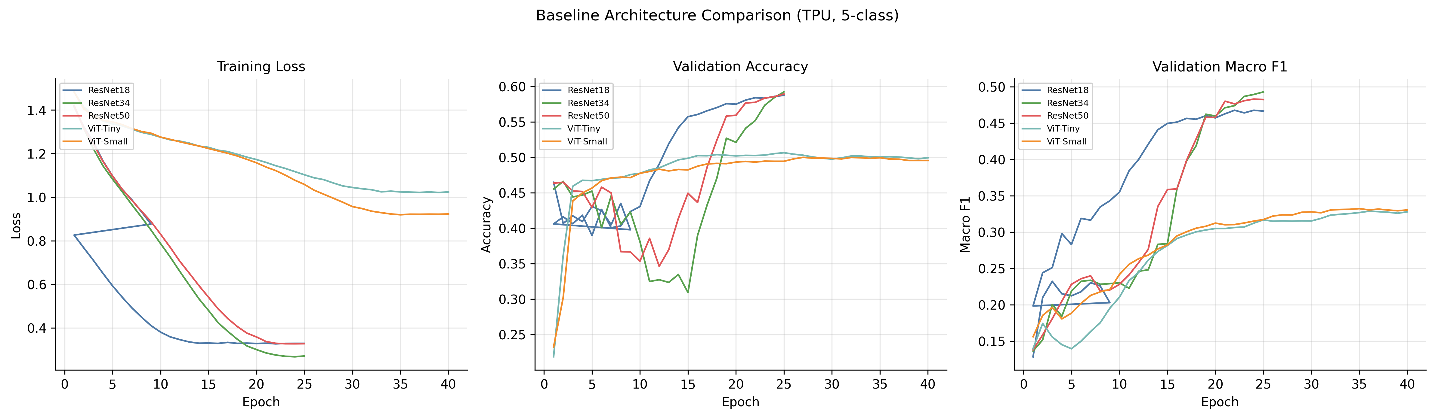
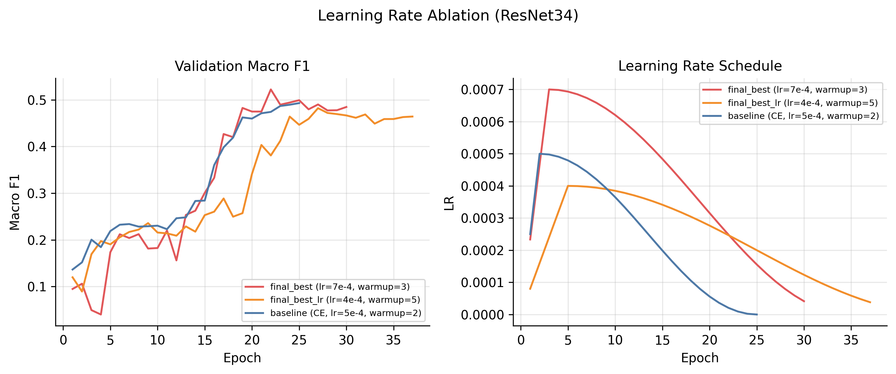
The convergence patterns split cleanly along architecture lines. ResNets descend smoothly. ViTs sit near chance for the first 5–10 epochs and then start learning. That is a now-familiar transformer warmup pattern that you have to budget compute for.
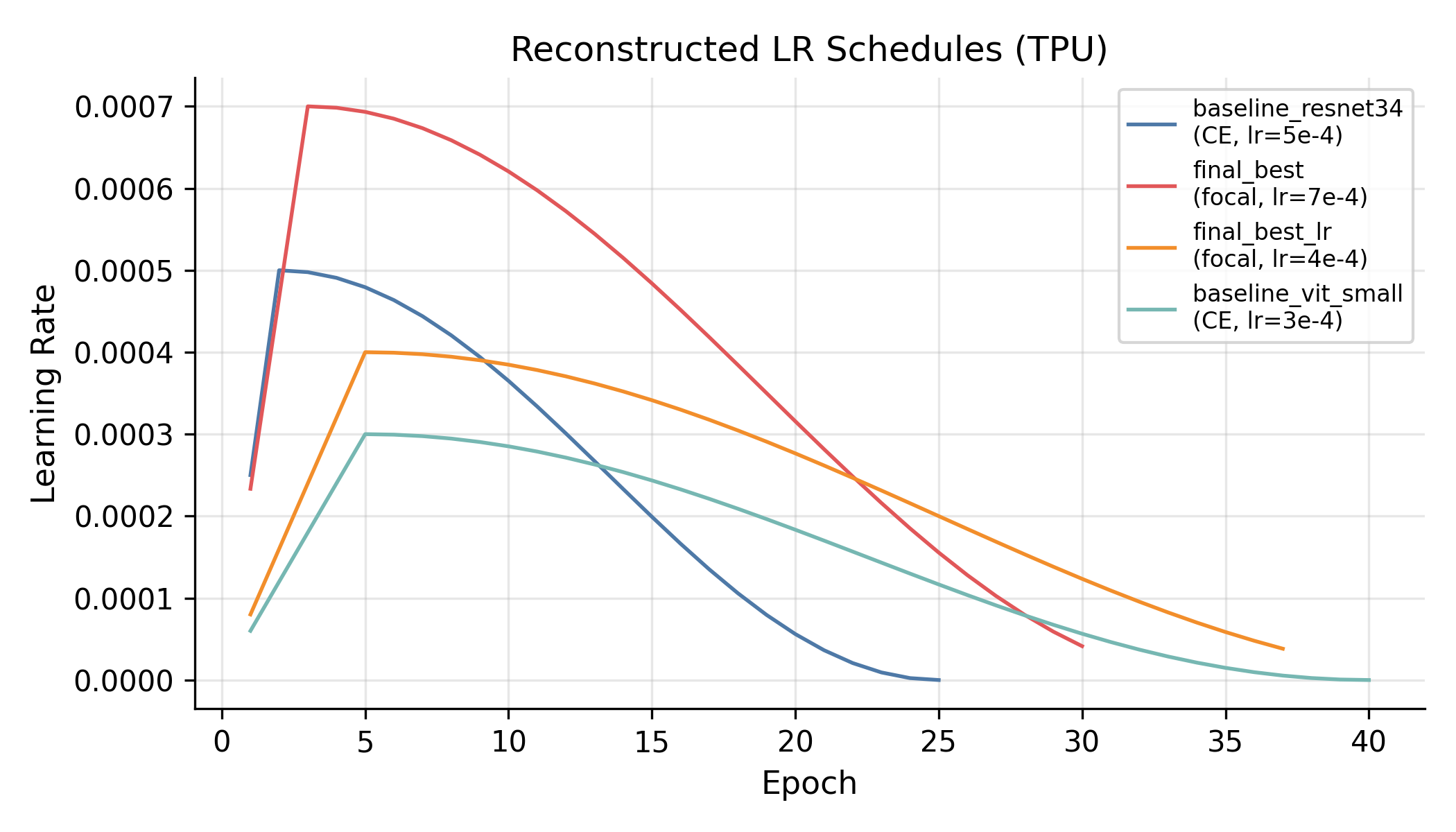
The schedule is the standard linear warmup → cosine decay; the figure above is reconstructed analytically from the configs because, embarrassingly, I had not logged the LR step-by-step during training. Lesson #1 for next time.
Baseline results, 5-class test set
| Architecture | Params | Test Acc. | Test Macro-F1 | Test ROC-AUC |
|---|---|---|---|---|
| ResNet18 | 11.2M | 0.410 | 0.231 | 0.662 |
| ResNet34 | 21.3M | 0.580 | 0.485 | 0.800 |
| ResNet50 | 21.3M | 0.584 | 0.481 | 0.801 |
| ViT-Tiny | 5.4M | 0.496 | 0.337 | 0.706 |
| ViT-Small | 21.5M | 0.514 | 0.372 | 0.720 |
Two things stand out immediately:
-
ResNets crush ViTs from scratch. The ViTs don’t have the inductive biases (locality, translation equivariance) that convolutions hand you for free, and on ~50k training images that gap is brutal. You can see it in the curves and you can see it in the final macro-F1: 11–15 pp behind ResNet34.
-
ResNet18 collapses on the small classes. Its 0.231 macro-F1 hides zero recall on
BENIGN_MASSandMALIGNANT_MASS. The validation curves wobble for the entire 25 epochs without ever stabilising. At this image scale, a ResNet18 just doesn’t have the capacity to resolve all five classes simultaneously.
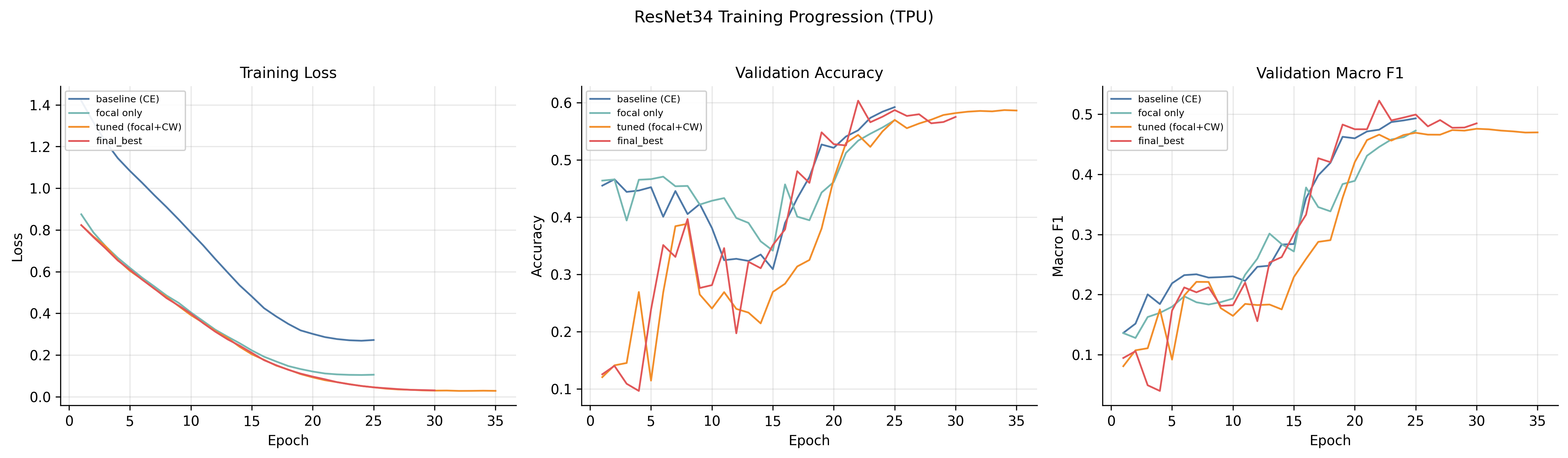
Tuning ResNet34: the slog
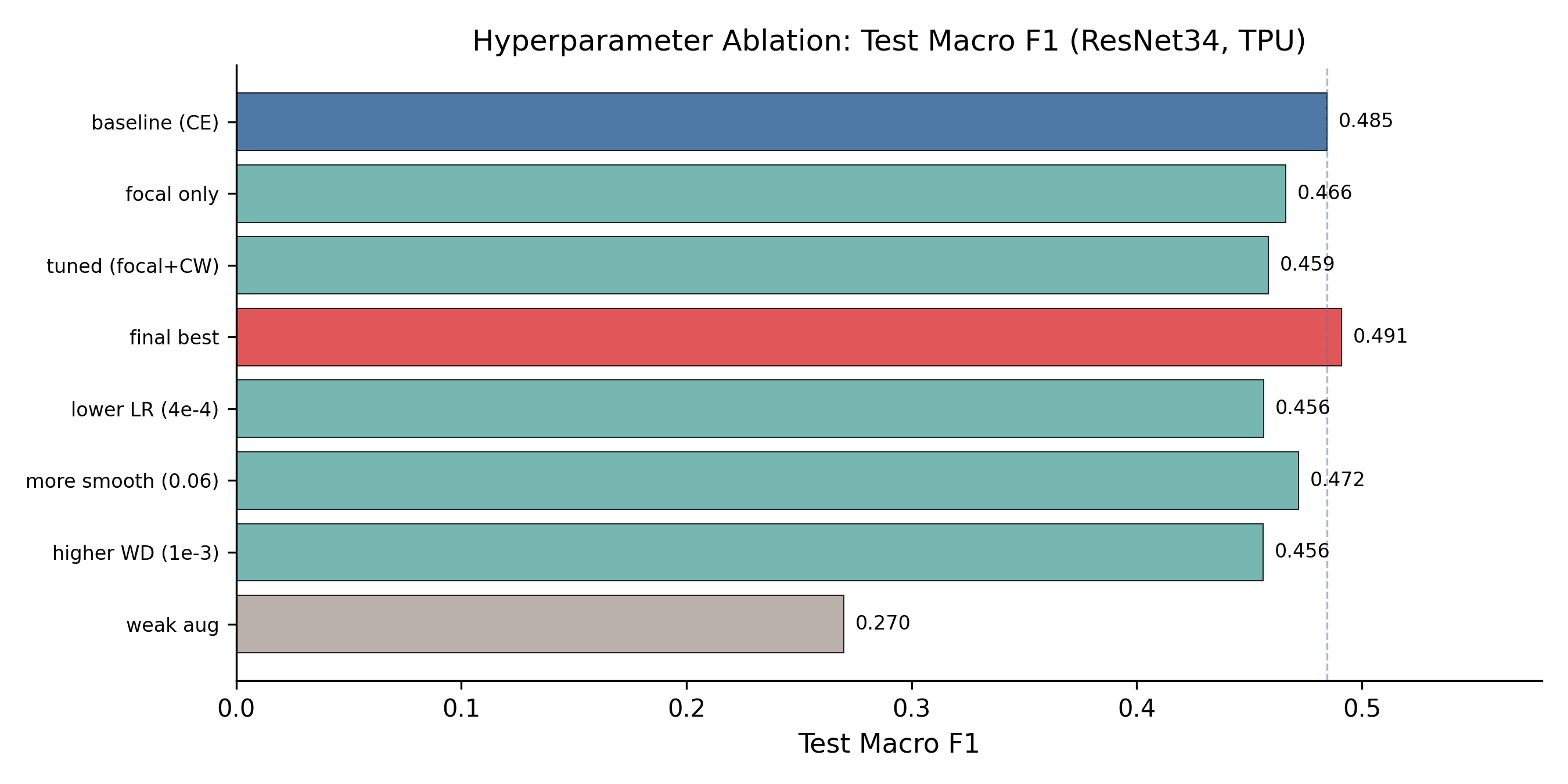
ResNet34 became the workhorse. I ran a small progression: cross-entropy baseline → focal loss only → focal + class weights + dropout + LR/WD tweaks → “final best”.
| Run | Loss | LR | Class Wt. | Test Macro-F1 |
|---|---|---|---|---|
| baseline | CE | 5e-4 | none | 0.485 |
| focal_only | Focal | 5e-4 | none | 0.466 |
| tuned | Focal | 7e-4 | [0.5, 1, 1, 1.3, 1.3] | 0.459 |
| final_best | Focal | 7e-4 | [0.5, 1, 1, 1.3, 1.3] | 0.491 |
The honest takeaway: I gained 0.6 percentage points of test macro-F1 over the cross-entropy baseline after a multi-week tuning campaign. The recipe matters, but the architecture mattered far more.
There’s also a humbling observation buried in this table. tuned and final_best share identical hyperparameters and the same random seed (21), yet differ by 3.2 pp on test macro-F1. This is TPU non-determinism: non-associative floating-point reductions across cores, XLA compilation choices that vary between runs, things like that. The variance band is comparable in size to the entire ablation range, which means some of the apparent ranking between hyperparameter variants is partially noise. If I were doing this again I would budget seeds the way I budget hyperparameters.
The augmentation surprise
The single most important hyperparameter in the entire study was data augmentation. Not learning rate, not weight decay, not loss function. Augmentation.
The “conservative” recipe is:
- random translation up to 6 pixels
- random rotation up to 10°
- brightness jitter δ = 0.05
- contrast jitter [0.95, 1.05]
- no horizontal flip (left/right asymmetry can be diagnostic in mammograms)
The “weak” recipe drops the translation to 4 pixels, the rotation to 8°, and removes brightness/contrast jitter entirely. That’s it. That is the full delta.
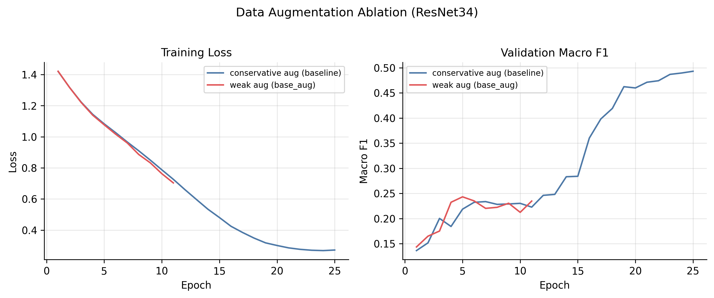
Weak augmentation collapsed the model from 0.485 to 0.270 test macro-F1, a 21.5 pp drop. The training loss curves tell the story: under weak augmentation, train loss falls faster (overfitting), validation macro-F1 plateaus below 0.25 and then declines, triggering early stopping at epoch 11. The model has the capacity to memorise the dataset, and removing two pixels of translation and the brightness jitter is enough to let it.
By comparison, every other single-factor ablation I ran lived inside a 3.5 pp range. Augmentation was an order of magnitude more impactful than every other knob put together.
Where the TPU pipeline lands overall
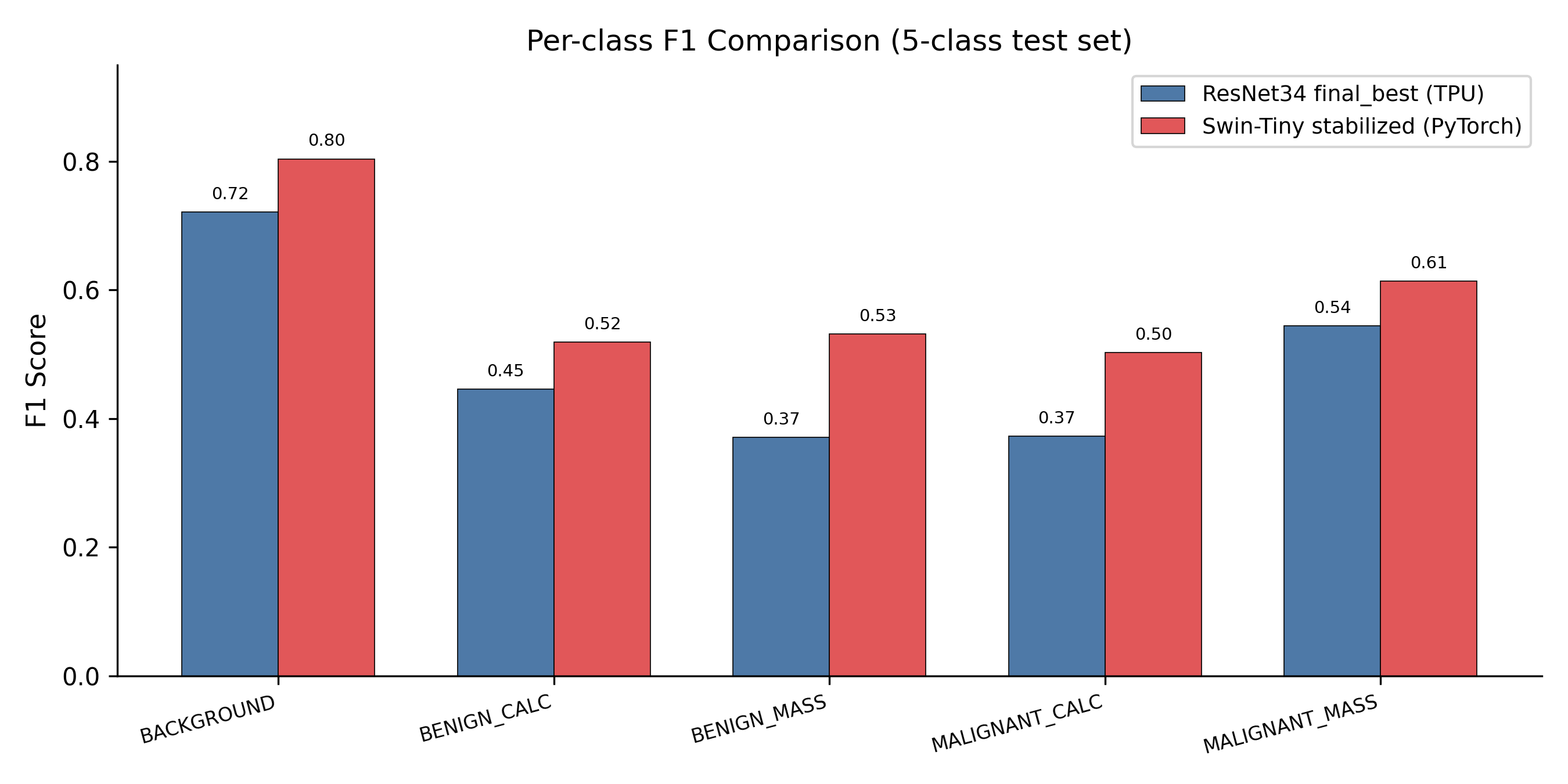
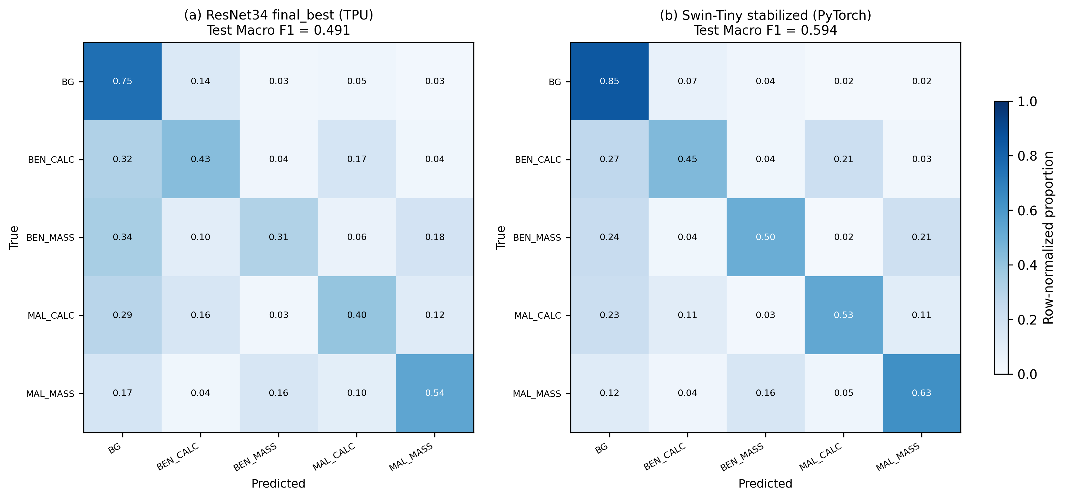
The best TPU model, ResNet34 final_best, reaches 0.491 test macro-F1 on the 5-class task. That’s a meaningful jump over the strongest classical baseline (PCA + HistGradientBoosting at 0.486 balanced accuracy on the easier 3-class task). But it is also clearly outclassed by the PyTorch pipeline once pretrained ImageNet weights enter the picture:
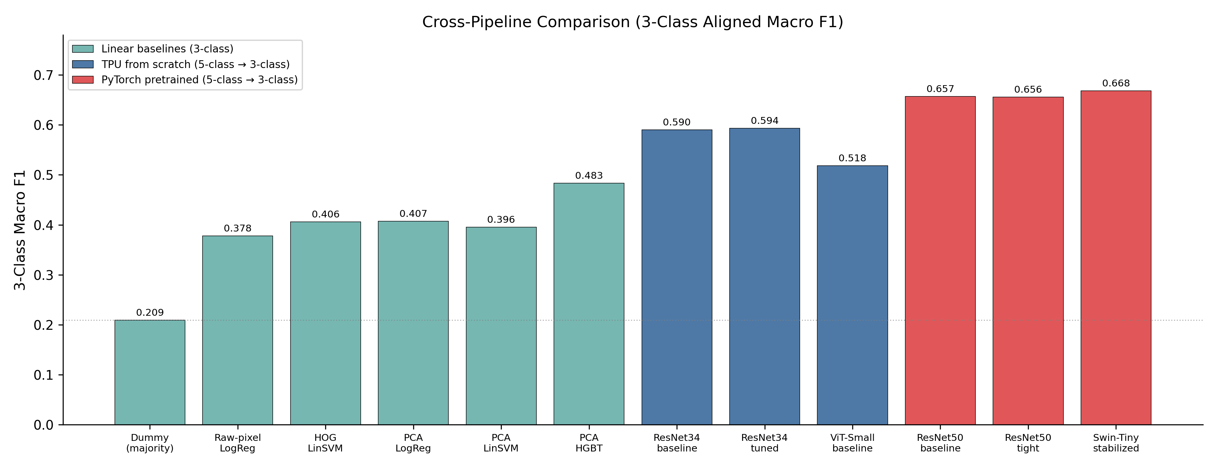
A Swin-Tiny stabilised on a single L40S GPU with ImageNet pretraining reaches 0.594 test macro-F1, a +10 pp gap over the best from-scratch TPU model. The gap shows up most strongly on the hardest, smallest classes: BENIGN_MASS (+16.1 pp) and MALIGNANT_CALCIFICATION (+13.0 pp). That is exactly where transfer learning is supposed to help.
Pretraining wins. Even features learned on natural images transfer remarkably well to grayscale mammographic patches when target data is limited. If clinical performance is the only thing you care about, you absolutely take the pretrained model. The reason to run the TPU pipeline anyway was that I wanted to learn the JAX/Flax/TPU stack from the inside, and the only honest way to learn it is to ship 15 real experiments through it.
Lessons I would carry into the next project
- Augmentation is a load-bearing hyperparameter. Treat it with the same rigor as the optimizer. A 2-pixel translation difference moved my macro-F1 by 21 percentage points.
- Budget seeds, not just configs. TPU non-determinism gave me a 3.2 pp run-to-run band on identical seeds. Reporting a single number for a single seed is dishonest at this scale; I should have run each “interesting” config 3–5 times.
- Log the LR you actually applied. Reconstructing schedules from configs after the fact works, but only because the schedule is deterministic. I got lucky.
- From-scratch on a small medical-imaging dataset is a hard mode you do not need to play. If the goal is clinical performance, start with pretrained weights and a sensible fine-tuning recipe. The from-scratch numbers are only worth chasing if the learning is the point, which, for me, it was.
- JAX/Flax on TPU is genuinely lovely once you internalise the functional pattern.
pmapmakes data parallelism legible. The painful parts are everything around training: pretrained weight loading, ONNX export, GradCAM. None of those exist as drop-in tools the way they do in PyTorch. Pick the stack that matches the problem. - Architecture > tuning, on small datasets. A multi-week ResNet34 tuning campaign moved the needle 0.6 pp. Switching to a pretrained Swin-Tiny moved it +10 pp. Choose your battles.
The TPU pipeline lives at Davidnet/CM3070-Models-Training-with-TPUs. Configs, training scripts, and the evaluation harness are all there.
If you have questions or spot something I got wrong, my contact details are on the front page.